Introduction
For designers seeking efficient workflows, our AI SVG Generator tools generate professional icons, logos, and illustrations from text descriptions—produce custom designs instantly with clean optimized paths and infinite scalability.
Scalable Vector Graphics (SVG) represents one of the most mathematically sophisticated image formats in modern web development. Unlike raster images that store pixel data, SVG leverages geometric primitives, parametric equations, and advanced algorithms to create infinitely scalable graphics. This comprehensive guide explores the mathematical foundations that power SVG technology, revealing how complex algorithms transform mathematical concepts into the visual elements we see on screen.
From the Bézier curve polynomials that create smooth paths to the affine transformation matrices that enable rotations and scaling, every aspect of SVG generation relies on sophisticated mathematical principles. Whether you're using our SVG generator to create graphics or building complex scalable vector graphics from scratch, understanding these algorithms provides crucial insight into optimizing performance and achieving precise visual results.
Mathematical Foundations of SVG Graphics
Vector Geometry and Coordinate Systems
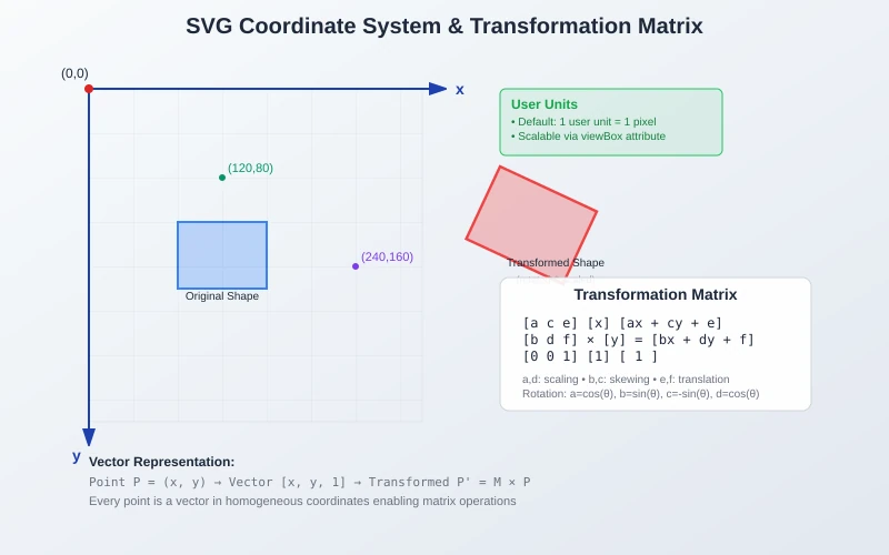
SVG employs a 2D Cartesian coordinate system where mathematical precision determines every visual element. The origin (0,0) sits at the top-left corner, with the positive x-axis extending rightward and the positive y-axis downward. This coordinate system uses floating-point precision, enabling sub-pixel accuracy crucial for high-quality rendering.
The mathematical relationship between points follows fundamental vector geometry principles. Every point P can be represented as a vector (x, y) in the coordinate space, where transformations operate through matrix operations. This vector-based approach enables SVG's resolution independence - shapes remain mathematically precise at any scale.
Key Mathematical Concepts:
- Coordinate Transformation: Points transform via matrix multiplication: P' = M × P
- User Units: Flexible measurement units that map to pixels or physical dimensions
- Continuous Plane: Mathematical curves exist in continuous space, not discrete pixels
- Linear Algebra: Vector operations underpin all coordinate manipulations
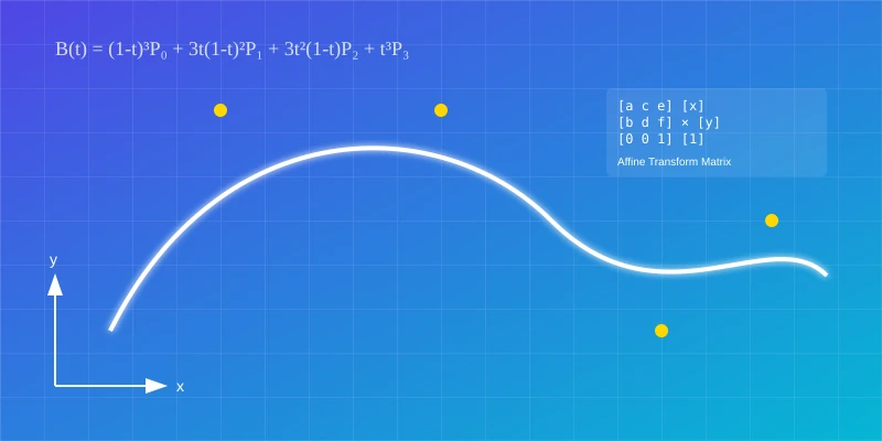
SVG transformations rely on 2D affine transforms represented by 3×3 homogeneous coordinate matrices. The general SVG transform matrix [a b c d e f] corresponds to:
M = | a  c  e |
    | b  d  f |
    | 0  0  1 |
This matrix performs the transformation: x' = ax + cy + e, y' = bx + dy + f
Transformation Types and Their Mathematical Representations:
- Translation: Moving elements using offset vectors
- Rotation: Circular transformations using trigonometric functions
- Scaling: Proportional resizing via multiplication factors
- Skewing: Angular distortion through shear transformations
Matrix multiplication enables transformation composition, where multiple operations combine into a single matrix for computational efficiency. This mathematical approach preserves lines and parallelism - fundamental properties for accurate vector rendering.
Bézier Curves: The Mathematical Foundation of Smooth Paths
Bézier curves form the mathematical backbone of SVG path generation. These parametric polynomial curves use control points to define smooth, scalable shapes through elegant mathematical formulations.
Quadratic Bézier Mathematics:
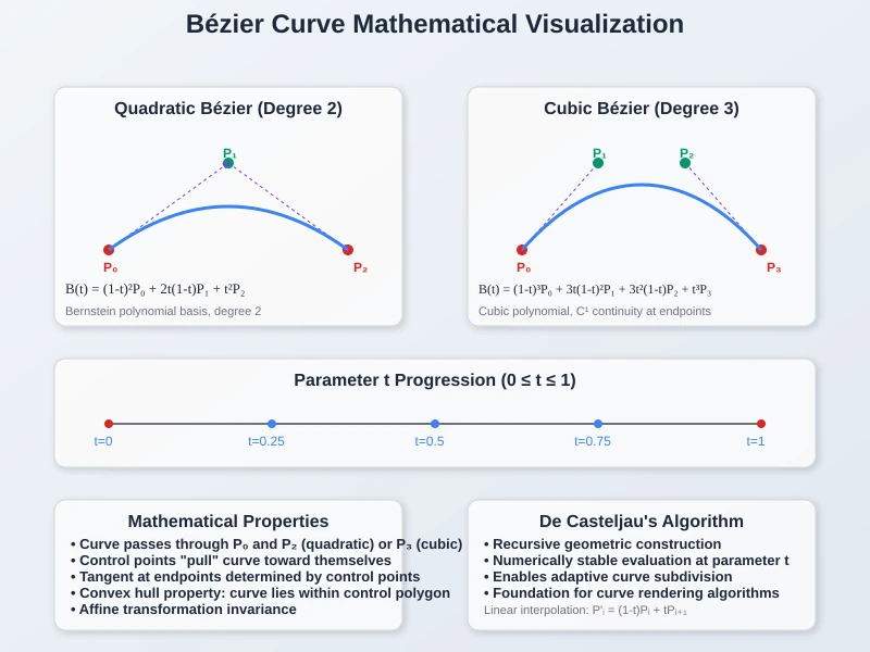
The quadratic Bézier curve connecting points P₀ to P₂ with control point P₁ follows:
B(t) = (1-t)²P₀ + 2t(1-t)P₁ + t²P₂, where 0 ≤ t ≤ 1
This expands to Bernstein polynomial basis functions of degree 2, providing C¹ continuity (continuous first derivative) at connection points.
Cubic Bézier Mathematics:
Cubic Bézier curves use four control points (P₀, P₁, P₂, P₃) with the mathematical formulation:
B(t) = (1-t)³P₀ + 3t(1-t)²P₁ + 3t²(1-t)P₂ + t³P₃
This degree-3 polynomial produces curves that start at P₀ (tangent to P₀-P₁) and end at P₃ (tangent to P₂-P₃). The intermediate control points "pull" the curve toward themselves without lying on the final path.
Advanced Bézier Properties:
- De Casteljau's Algorithm: Recursive geometric construction for curve subdivision
- Control Point Reflection: Automatic smooth curve continuation using reflected control points
- Curve Continuity: Mathematical guarantees for smooth path connections
- Error Bounds: Quantifiable approximation accuracy for curve fitting
Parametric vs. Implicit Curve Representations
SVG primarily uses parametric equations where coordinates express as functions of parameter t. This approach contrasts with implicit representations (F(x,y) = 0) used in analytical geometry.
Parametric Advantages for SVG:
- Rendering Efficiency: Direct point sampling by iterating parameter t
- Tangent Computation: Derivatives provide curve direction for animation
- Arc Length Parameterization: Essential for text-on-path and motion animations
- Numerical Stability: Better computational properties for graphics algorithms
Examples of Parametric Forms:
- Line: L(t) = (1-t)P₀ + tP₁
- Circle: C(θ) = (r cos θ, r sin θ)
- Ellipse: E(θ) = (a cos θ cos φ - b sin θ sin φ, a cos θ sin φ + b sin θ cos φ)
Advanced Algorithms for SVG Path Rendering
Curve Tessellation and Adaptive Subdivision
Converting smooth parametric curves to discrete pixel representations requires sophisticated tessellation algorithms. The de Casteljau algorithm provides mathematically robust curve subdivision:
Algorithm Steps:
- Flatness Testing: Measure deviation between curve and straight line approximation
- Recursive Subdivision: Split curves exceeding flatness tolerance
- Convergence Guarantee: Subdivision continues until error bounds are met
- Pixel-Level Accuracy: Final segments approximate curves within one device pixel
Mathematical Foundations of Path Operations
Boolean Path Operations:
Complex shape combinations rely on computational geometry algorithms:
- Union: Combining multiple paths using winding number calculations
- Intersection: Finding overlapping regions through line segment intersection algorithms
- Difference: Subtracting paths using even-odd fill rules
- XOR: Symmetric difference operations for complex shape creation
Winding Number Mathematics:
The mathematical determination of point-inside-path uses ray-casting algorithms with signed crossing counts:
Winding Number = Σ(signed crossings) / 2π
Vectorization: Converting Raster to Vector Mathematics
Edge Detection Algorithms
Raster-to-vector conversion begins with mathematical edge detection using convolution operators:
Sobel Operator Mathematics:
Gx = |−1  0  1|     Gy = |−1 −2 −1|
     |−2  0  2|          | 0  0  0|
     |−1  0  1|          | 1  2  1|
Gradient Magnitude: |G| = √(Gx² + Gy²)
Gradient Direction: θ = arctan(Gy/Gx)
The Potrace algorithm provides mathematically optimal bitmap tracing through sophisticated optimization:
Algorithm Phases:
- Path Decomposition: Convert binary bitmap to closed polygonal paths
- Polygon Optimization: Dynamic programming for minimal vertex count
- Corner Detection: Identify sharp direction changes requiring curve breaks
- Curve Fitting: Least-squares optimization for Bézier approximation
Mathematical Optimization:
Potrace minimizes the cost function:
Cost = Σ(point-to-curve distance²) + λ(complexity penalty)
Procedural SVG Generation Through Mathematical Functions
For rapid design iteration, our AI SVG Generator generates multiple design variations from text prompts in seconds—create matching icons, logos, and graphics instantly with consistent styling across all your mathematical and procedural projects.
Fractal Mathematics in SVG
Fractal generation leverages mathematical recursion and self-similarity for infinite detail:
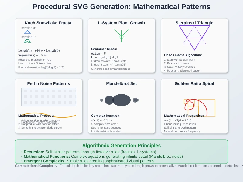
Koch Snowflake Algorithm:
Initial: Triangle
Iteration n: Replace each line segment with 4 segments forming a "spike"
Mathematical Growth: 4ⁿ segments after n iterations
Mandelbrot Set Mathematics:
For point c in complex plane:
z(n+1) = z(n)² + c
Fractal Membership: |z| remains bounded as n → ∞
L-Systems: Algorithmic Plant Generation
Lindenmayer Systems use formal grammar rules for organic shape generation:
Mathematical Foundation:
- Alphabet: Symbols representing drawing commands (F=forward, +=turn right, -=turn left)
- Production Rules: Symbol replacement rules (F → F+F--F+F)
- Iteration: Recursive string rewriting creates complex patterns
Example - Fractal Plant:
Axiom: F
Rule: F → F[+F]F[-F]F
Iterations: F → F[+F]F[-F]F → F[+F]F[-F]F[+F[+F]F[-F]F]F[+F]F[-F]F[-F[+F]F[-F]F]F[+F]F[-F]F
Perlin Noise for Organic Patterns
Ken Perlin's noise algorithm generates mathematically controlled randomness:
Algorithm Components:
- Gradient Vectors: Pseudo-random unit vectors at lattice points
- Interpolation: Smooth transitions using fade functions (6t⁵-15t⁴+10t³)
- Octave Summation: Fractal Brownian motion through frequency layering
Mathematical Formula:
Noise(x,y) = Σ(amplitude_i × noise_i(frequency_i × x, frequency_i × y))
SVG Path Optimization: Mathematical Simplification
Ramer-Douglas-Peucker Algorithm
This mathematical algorithm optimally reduces path complexity while preserving shape fidelity:
Algorithm Logic:
- Line Approximation: Draw straight line between path endpoints
- Maximum Deviation: Find point with greatest perpendicular distance to line
- Recursive Decision: If distance > tolerance, subdivide; otherwise, eliminate intermediate points
- Optimal Result: Minimal points for given error tolerance
Mathematical Guarantee:
The algorithm minimizes vertex count while ensuring maximum approximation error stays below threshold ε.
Curve Fitting Mathematics
Schneider's Algorithm provides least-squares optimization for Bézier curve fitting:
Optimization Objective:
Minimize: Σ|P(t_i) - B(t_i)|²
Subject to: B(t) = cubic Bézier with optimal control points
Iterative Refinement:
- Parameter optimization through Newton-Raphson iteration
- Control point adjustment via linear algebra
- Error measurement using L² distance metrics
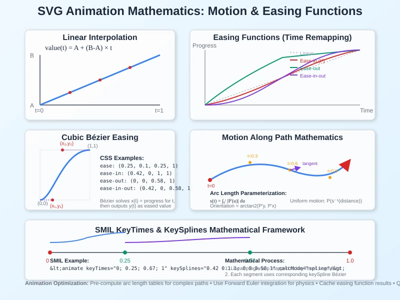
Animation Mathematics: Motion and Easing Functions
Interpolation Mathematics
SVG animations rely on mathematical interpolation between keyframe values:
Linear Interpolation:
value(t) = A + (B-A) × (t-t₀)/(t₁-t₀)
Bézier Easing Functions:
CSS and SMIL use cubic Bézier curves for time remapping:
Easing(t) = CubicBézier(0,0, x₁,y₁, x₂,y₂, 1,1)
Common easing functions:
- ease-in: (0.42, 0, 1, 1) - quadratic acceleration
- ease-out: (0, 0, 0.58, 1) - quadratic deceleration
- ease-in-out: (0.42, 0, 0.58, 1) - combined acceleration/deceleration
Path Motion Mathematics
Arc Length Parameterization:
For motion along arbitrary paths, uniform speed requires arc length calculation:
s(t) = ∫₀ᵗ |P'(u)| du (total arc length)
Motion Position: P(s⁻¹(distance_traveled))
Orientation Mathematics:
Auto-rotation along paths uses tangent vector calculations:
Tangent = P'(t)
Orientation = arctan2(P'_y(t), P'_x(t))
Advanced SVG Filter Mathematics
Convolution Mathematics
SVG's feConvolveMatrix implements discrete convolution for image processing:
Mathematical Formula:
Output(x,y) = ΣΣ Input(x+i, y+j) × Kernel[i,j]
Common Kernels:
- Gaussian Blur: G(x,y) = (1/2πσ²)e^(-(x²+y²)/2σ²)
- Edge Detection: Sobel, Prewitt, and Laplacian operators
- Sharpening: Center-weighted kernels emphasizing high frequencies
Color Space Mathematics
RGB Color Matrix Transformations:
[R'] = [r₁₁ r₁₂ r₁₃ r₁₄ r₁₅] [R]
[G']   [r₂₁ r₂₂ r₂₃ r₂₄ r₂₅] [G]
[B'] = [r₃₁ r₃₂ r₃₃ r₃₄ r₃₅] [B]
[A']   [r₄₁ r₄₂ r₄₃ r₄₄ r₄₅] [A]
[1]    [ 0   0   0   0   1 ] [1]
Luminance Calculation:
Grayscale = 0.2126×R + 0.7152×G + 0.0722×B
Hue Rotation Mathematics:
Hue shifts use rotation matrices in color space, involving sine and cosine calculations for angular transformations.
Our AI-powered svg generator lets designers create graphics through streamlined workflows—generate custom icons, logos, and illustrations that apply sophisticated mathematical algorithms without requiring deep technical knowledge.
D3.js Mathematical Foundations
D3's data visualization relies heavily on mathematical interpolation and scaling:
Scale Functions:
- Linear Scale: y = mx + b (affine transformation)
- Log Scale: y = log_base(x) transformation
- Power Scale: y = x^exponent transformation
Curve Interpolation:
- curveBasis: Uniform cubic B-spline implementation
- curveCardinal: Catmull-Rom spline with tension parameter
- curveMonotoneX: Monotonic cubic interpolation preventing overshoots
Force Simulation Mathematics:
- Spring Forces: F = -kx (Hooke's Law)
- Coulomb Repulsion: F = k(q₁q₂)/r²
- Verlet Integration: Numerical integration for particle physics
Inkscape's Mathematical Algorithms
Inkscape implements numerous computational geometry algorithms:
Spiro Splines:
Mathematical curves minimizing curvature variation using clothoid segments (Cornu spirals). The optimization involves solving differential equations for G² continuity.
Boolean Operations:
Path combinations using the Bentley-Ottmann algorithm for line segment intersection detection, combined with winding number calculations for interior/exterior determination.
Envelope Deformation:
Bilinear interpolation for shape warping:
P(u,v) = (1-u)(1-v)P₀₀ + u(1-v)P₁₀ + (1-u)vP₀₁ + uvP₁₁
Typography Mathematics in SVG
Font Outline Mathematics
Font rendering involves complex curve mathematics:
TrueType Outlines:
- Quadratic Bézier curves for glyph boundaries
- Coordinate system transformations (font units → user units)
- Hinting mathematics for pixel-grid alignment
Glyph Positioning Mathematics:
- Advance Width: Horizontal spacing between characters
- Kerning: Pairwise spacing adjustments using lookup tables
- Baseline Calculation: Vertical positioning using font metrics
Text-on-Path Mathematics:
Character placement requires arc length parameterization:
Character_Position = Path.getPointAtLength(accumulated_advance)
Character_Rotation = Path.getTangentAtLength(accumulated_advance)
Computational Complexity
Path Simplification Complexity:
- Douglas-Peucker: O(n log n) average case, O(n²) worst case
- Curve Fitting: O(n³) for least-squares optimization
- Subdivision Algorithms: O(log(1/ε)) for desired precision ε
Rendering Complexity:
- Tessellation: O(n) for adaptive subdivision depth n
- Rasterization: O(pixels × samples) for anti-aliasing
- Transform Composition: O(1) per matrix multiplication
Memory Optimization Mathematics
Path Coordinate Quantization:
Balancing precision vs. file size through controlled rounding:
Quantized_Value = round(Original_Value × 10^precision) / 10^precision
Bezier Degree Reduction:
Mathematical algorithms for approximating higher-degree curves with lower-degree alternatives, reducing computational load while maintaining visual fidelity.
Advanced Machine Learning in SVG Generation (2025 Update)
Neural Network-Based Vectorization
As of October 2025, deep learning has revolutionized SVG generation through sophisticated neural architectures:
DeepSVG - Hierarchical Generative Networks:
The DeepSVG model (NeurIPS 2020) represents a breakthrough in hierarchical generative networks for vector graphics. This system learns to accurately reconstruct diverse vector graphics and serves as a powerful animation tool through interpolations and latent space operations. It enables differentiable operations on SVG tensors, allowing gradient descent-based optimization to deform shapes matching arbitrary targets.
SVGformer - Transformer-Based Representation:
The latest SVGformer architecture (CVPR 2023) applies transformer models to continuous vector graphics representation learning. Unlike earlier approaches, SVGformer addresses the unique challenges of handling continuous SVG inputs, achieving superior performance in capturing intricate patterns and dependencies within large datasets.
Loss Functions:
Combining multiple mathematical objectives:
Loss = λ₁×Reconstruction_Error + λ₂×Smoothness_Penalty + λ₃×Complexity_Cost
Differentiable Rendering:
Modern techniques enable gradient-based optimization of vector graphics through neural networks, allowing end-to-end training of SVG generation systems.
Advanced Generative Models (2025)
Convolutional Variational Autoencoders (CVAEs):
State-of-the-art SVG generation now employs class-conditioned CVAEs - generative models that learn to encode data into lower-dimensional latent spaces and decode back to original form. By harnessing CNNs and VAEs, these systems demonstrate remarkable capabilities in capturing intricate patterns within large graphics datasets, particularly for fonts and icons.
Generative Adversarial Networks (GANs):
Mathematical competition between generator and discriminator networks:
min_G max_D E[log(D(x))] + E[log(1-D(G(z)))]
Modern GANs achieve unprecedented quality in SVG generation, with adversarial training producing crisp, professional vector outputs indistinguishable from human-created graphics.
Variational Autoencoders (VAEs):
Probabilistic models for structured SVG generation using latent space mathematics. These advanced algorithms power text to SVG transformation by converting semantic understanding into vector representations, enabling intuitive text-to-vector workflows used by millions of creators worldwide in 2025.
Conclusion
For designers who prefer describing concepts, AI Text to SVG tools transform your design ideas into production-ready vector graphics—generate custom icons and illustrations instantly from plain text without mastering complex mathematical algorithms.
The mathematical foundations underlying SVG generation represent a sophisticated blend of computational geometry, linear algebra, numerical analysis, and algorithmic optimization. From the parametric polynomials defining Bézier curves to the matrix transformations enabling complex animations, every aspect of SVG relies on rigorous mathematical principles.
Understanding these algorithms enables developers and designers to:
- Optimize Performance: Choose appropriate algorithms for specific tasks
- Ensure Quality: Apply mathematical precision to visual design
- Innovate Solutions: Develop new techniques building on established foundations
- Debug Effectively: Understand why specific approaches succeed or fail
As generative SVG technology continues evolving, these mathematical foundations remain constant. Whether creating simple icons or complex data visualizations, the algorithms discussed here power every pixel-perfect, infinitely scalable graphic we see today.
The intersection of mathematics and visual design in SVG demonstrates how abstract algorithmic concepts translate into practical, beautiful, and functional graphics. As we advance toward more intelligent SVG generation systems and sophisticated vector graphics tools, these mathematical principles will continue serving as the bedrock for innovation in computational graphics.
Experience these mathematical algorithms in action with our ai svg generator - where complex computational geometry meets intuitive design, allowing you to create mathematically precise vectors through simple prompts.
External References and Further Reading
For deeper exploration of the mathematical concepts discussed: